Tools Menu
The Tools Menu offers the following commands:

The Zoom command selects the zoom tool as the current tool.
To zoom in on a specific point, choose the [Zoom tool] from the toolbar or, [Tool/Zoom] from menu bar. A magnifying glass icon should appear on the screen. To zoom in, left click without dragging the mouse. The view is centered on where the mouse was clicked and will zoom in by a factor of two. To zoom out, right click without dragging the mouse. The view will zoom out by a factor of two, centered on where the mouse was clicked. You can also hold down the Ctrl key while right clicking to restore the view to the last zoomed view.
Alternately, one can zoom in to a user-defined rectangle by left clicking and then draging a box while holding down the left mouse button.
If your mouse has a middle button, you can hold it down and drag the map similar to the behavior of the Pan (Grab-and-Drag) tool.
Pan (Grab-and-Drag) Tool
The Pan (Grab-and-Drag) command selects the Pan tool as the current tool.
To change the center point of the image without changing the magnification, depress the left mouse button, drag the view to the desired location, then release the left mouse button to redraw the view at the new location.
If you just want to recenter on a new location without dragging, just click the left mouse button at the new desired location and the view will be recentered on that location (this provides the functionality of the old Recenter Tool).
Measure Tool
The Measure command selects the measure tool as the current tool.
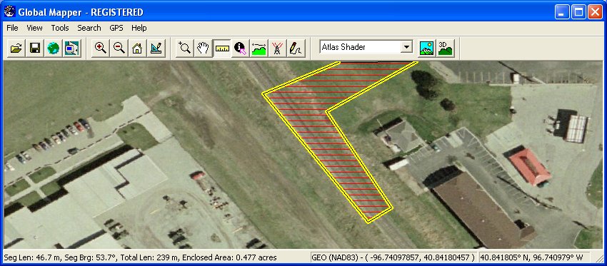
To find the distance between along a path on the display or the enclosed area of a set of points, choose the [Measure Tool] icon from the toolbar or select [Tools/Measure] from the menu bar.
Note that if you place a point along your measurement that you do not want you can press Ctrl+Z to remove the last placed point in the measurement.
You can also save a measurement to a separate feature by right clicking and selecting "Save Measurement" from the list that pops up. You can then export these measurements to new vector files, such as Shapefiles or DXF, or modify them with the Digitizer Tool. There is also an option to copy the measurement text to the clipboard when you right-click.
If you have gridded elevation data loaded under the measurement, you can also calculate the Cut-and-Fill volume either within the measurement area or within some distance of the measurement line. To do this, simply right click then select the "Measure Volume (Cut-and-Fill)" option that appears. Selecting this option will display the Setup Volume Calculation Parameters dialog (pictured below), which allows you to set up the volume measurement.
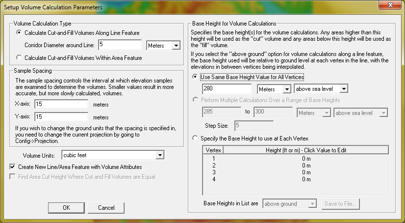
On the Setup Volume Calculate Parameters you can select whether to measure cut-and-fill volumes within some specified distance of the selected line or within the specified area. If you are measuring along a line, you can specify the cut heights to use at each vertex individually or use the same cut (base) height for each vertex relative either to the ground at each vertex or relative to sea level. Whichever option you choose, the heights will be interpolated between line vertices to get a smoothly varying cut height. If measuring within an area, there is also an option to perform multiple cut-and-fill calculations between a range of cut (base) height values. If you choose this option the results will be displayed in a table at the end of the operation so you can see the results of each calculation.
Once you have your volume calculation setup and you press ok to calculate it, the volume of earth that would be needed to fill any space below the cut surface (fill volume) is reported along with the volume of earth that is above the cut surface (cut volume). After viewing the reported volumes, you have the option to save a new feature with the measurement values.
If measuring the cut-and-fill volumes within an area feature, you can also check the Find Area Cut Height Where Cut and Fill Volumes are Equal to find the approximate cut height where the same amount of dirt would have to be cut out as filled. This is useful for selecting a cut height at which no dirt needs to be hauled off or brought in. The optimal cut height will be reported as the break-even height with the other measurement results.
On the right-click menu in the Measure Tool are options to control how distances are measured and the paths are drawn. The following options are available:

The Feature Info command selects the Feature Information tool as the current tool. This tool allows you to select vector features (areas, lines, and points) by clicking on or near them. Once selected, a dialog displaying information about the selected item appears.
To pick objects, select the [Feature Info] icon from the Toolbar or select [Tools/Feature Info] from the menu bar. Press and release the left mouse button near the objects(s) to be picked. Holding down the 'P' key when left clicking causes only area features at the clicked location to be considered. If left-clicking on a picture point with an associated image, by default just the image will be displayed, but holding the Ctrl key when clicking will cause the normal feature info dialog to be displayed. When an object is picked, it will be highlighted and a feature info dialog (picture below) will be displayed. Right clicking the mouse button cycles through each of the elements located near the selection point, displaying the information in the dialog box.
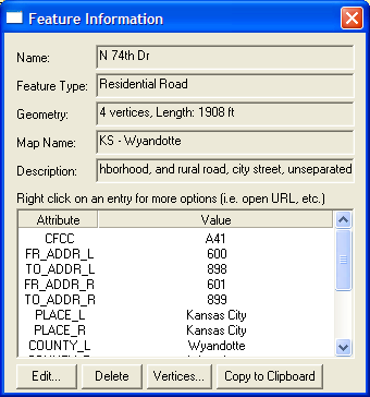
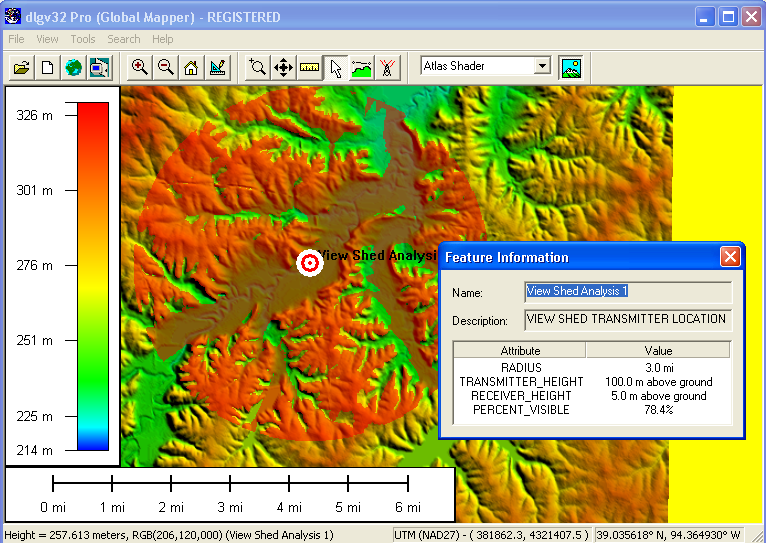
As you can see, you can view a lot of information about a selected object in the Feature Info dialog. The object's name, description, geometry information including length and enclosed area (when applicable), attribute value list, and map name, are all displayed. Buttons are also available allowing you to edit the selected feature's information and drawing style, marking the selected feature as deleted, as well as to copy all of the feature information (as text) and the feature itself to the Windows clipboard for pasting elsewhere, such as in a text editor or as a new feature in a running session of Global Mapper.
In addition, you can right click on any attribute value to see additional options specific to the selected attribute/value pair. You can copy the selected pair to the Windows clipboard, treat the value as a web URL and open that location in a web browser, or treat the value as a filename (either absolute or relative to the path of the source file from which the feature was read) and load that file either into Global Mapper or with the program associated with that file type in Windows. You can also choose to zoom the main map view to the extents of the selected feature.
If the selected feature has an attribute named IMAGE_LINK and the value of that attribute refers to a local image file, Global Mapper will automatically open that image in the associated application on your system, unless the Ctrl button was held down when you selected the feature. Likewise if you have an attribute named GM_LINK and the value of that attribute refers to a local file, Global Mapper will try and open that file in the current instance of Global Mapper as a new layer, unless the layer is already open or the Ctrl key was held down.
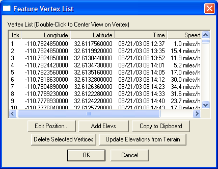
Clicking the Vertices button for line or area features displays the Feature Vertex List dialog (pictured below), which allows you to view, edit, and remove the individual vertex coordinates, including Z and timestamp values (if present) for the selected feature. The X and Y coordinates are listed in the native projection of the layer, and the Z coordinates will have the elevation units defined for the layer on the Projection tab of the Options dialog for the layer. You can also easily add per-vertex elevation values to features that do not already have them by pressing the Add Elevs button on the Feature Vertex List dialog. If timestamp values are present (like for a GPS tracklog), speed and bearing columns will also be displayed for each leg of the feature. You can also right-click on the vertex list for a feature with per-vertex elevations and choose the option to evenly spread the elevations to achieve a constant slope between the first and last elevation on the feature and also to replace any zero elevation values by interpolating between non-zero values. You can also add and edit per-vertex timestamps by right-clicking on the vertex list and selecting the appropriate option.

The PathProfile/LOS command selects the 3D path profile/LOS (line of sight) tool as the current tool. This tool allows you to get a vertical profile along a user-specified path using loaded elevation datasets. In addition, registered users can perform line of sight calculations along the defined path.
To define the path along which to generate the 3D path profile, first select the path profile tool as your current tool. Press and release the left mouse button at the position where you wish to start the path. Move the mouse to the next position that you want to include in the path profile, then press the left mouse button again. Right click on the last location in the path profile to complete selecting points and display the Path Profile/Line of Sight dialog (pictured below). The Path Profile/Line of Sight dialog will appear displaying the 3D path profile of the selected path. Any points along the path that did not have elevation data underneath will be treated as an elevation of zero.
You can also generate 3D path profiles for existing line features by selecting the line feature in the Digitizer Tool, right clicking, then selecting the Generate Path Profile From Line option on the menu that is displayed.
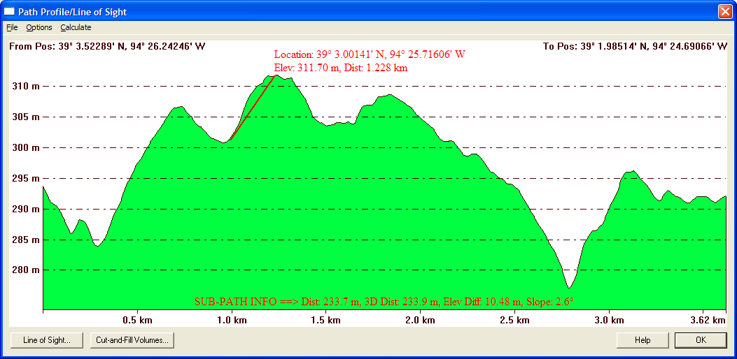
The Path Profile/Line of Sight dialog displays the 3D path profile and provides several options related to the profile. A vertical scale is displayed on the left hand side of the profile window. The start and end coordinates of the path are displayed at the top of the profile window. If more than two points are in the path, the intermediate points will be marked in the profile window with a yellow dot. These intermediate points can be toggled on and off using an option available by right clicking on the path profile window. Also note that this dialog is resizable. If you have water display enabled on the Vertical Options tab of the Configuration dialog and there would be water along the path, that will be displayed as well.
Moving your cursor over the profile window displays information about the current cursor location along the profile, including the position and profile elevation at the cursor location. You can get information about a portion of the profile (a sub-path) by left clicking to start a sub-path definition, then left-clicking again at the end of your desired sub-path. Details about the sub-path, like length, elevation change, and slope, will then be displayed on the bottom of the profile window.
Right clicking on the profile window brings up an options menu allowing the user to change the start and end positions, select the units (meters or feet) to display the elevations in, configure display of the path profile, and display a dialog containing details about the path. These options are also available under the Options menu on the dialog.
The File menu contains options allowing you to save the path profile/line of sight data to a file. The individual options are described below.
The Save To Bitmap... option allows registered users to save the contents of the path profile window to a Windows bitmap (BMP) file for use in other applications.
The Save to BMP and Display on Main Map View option allows registered users to save the contents of the path profile window to a Window bitmap (BMP) file and then display that BMP at a fixed location on the main map view. This is the equivalent of using the Save to Bitmap menu command, then closing the dialog and using the File->Open Data File at Fixed Screen Location menu command in the main map view.
The Save CSV File (with XYZ and Distance Values... option allows registered users to save all of the coordinates and distances to that location along the path profile to a CSV text file. Each line in the text file will be formatted as follow:
x-coordinate,y-coordinate,elevation,distance-from-start
The Save Distance/Elevation... option allows registered users to save all of the distances and elevations along the path profile to a text file. Each line in the text file will be formatted as follow:
distance-from-start,elevation
The Save To XYZ... option allows registered users to save all of the positions and elevations along the path profile to a text file. Each line in the text file will be formatted as follow:
x-coordinate,y-coordinate,elevation
The Save LOS to KML... option allows registered users to save a 3D line of sight and, if selected, the Fresnel zone boundary lines, to a KML file for display in Google Earth.
Pressing the Line of Sight... button brings up the Setup Line of Sight/Earth Curvature dialog (pictured below), which allows the user to configure a line of sight calculation along the selected path. You can only perform a line of sight analysis if exactly two points are in the path profile (e.g. line of sight analysis cannot be performed on multi-segment paths).
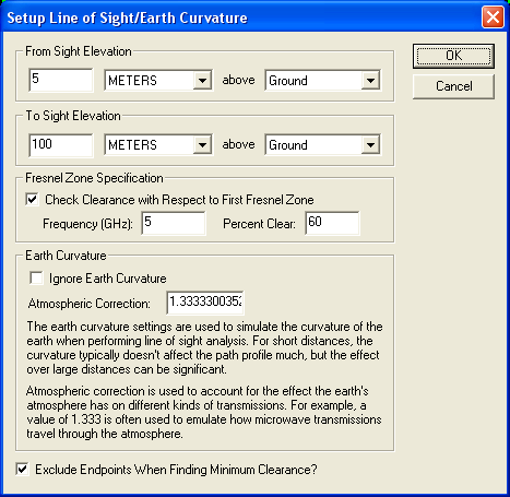
The From Sight Elevation section allows the user to select the height at the start position (left side of graph) to use in the line of sight calculations. This height can be specified in either feet or meters above the ground or above sea level. The To Sight Elevation section provides the same functionality for the end position (right side of graph).
The Fresnel Zone Specification section allows you to have the line of sight analysis also check that a certain portion (the Percent Clear value) of the first Fresnel zone for a transmission of a particular frequency is clear. The typical standard is that good visibility requires that at least 60% (the default) of the first Fresnel zone for the specified frequency be clear of obstructions. If Fresnel zone clearance is being selected the specified percentage of the first Fresnel zone will be drawn on the line of sight analysis dialog as a dotted line underneath the straight sight line.
The Earth Curvature section allows the user to specify whether they want to take the curvature of the earth into account while performing the line of sight calculation. In addition, when earth curvature is being used, they can specify an atmospheric correction value to be used. The atmospheric correction value is useful when determining the line of sight for transmitting waves whose path is affected by the atmosphere. For example, when modeling microwave transmissions a value of 1.333 is typically used to emulate how microwaves are refracted by the atmosphere.
Selecting the Exclude Endpoints when Finding Minimum Clearance options causes the first and last 5% of the elevations along the profile to be ignored when finding the minimum clearance point.
After setting up the line of sight calculation in the dialog and pressing the OK button, the line of sight will be displayed in the path profile window (pictured below). Along with the line depicted the actual line of sight, the position and vertical separation of the minimum clearance of the line of sight will be displayed with a dashed red line in the path profile window.

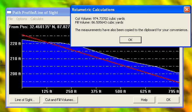
Pressing the Cut-and-Fill Volumes... button brings up the Setup Volume Calculation Parameters dialog, allowing the user to perform a cut-and-fill volume analysis along the path using loaded terrain data. See the Measure Tool for more information on cut-and-fill volume setup.
Once you have performed a cut-and-fill analsyis, the cut line will be displayed on the path profile allowing easy visualization of the cut and fill areas along the path, as evidenced by the picture below.

The View Shed command selects the view shed analysis tool as the current tool. This tool allows registered users to perform a view shed analysis using loaded elevation grid data with a user-specified transmitter location, height, and radius. All areas within the selected radius that have a clear line of sight to the transmitter are colored with a user-specified color.
To perform a view shed analysis, first select the view shed tool as your current tool. Press and release the left mouse button at the position where you wish to place the transmitter. At this point, the View Shed Setup dialog (pictured below) will appear, allowing you to setup the view shed calculation.
You can also calculate views sheds at multiple point locations by selecting the point features at the desired locations in the Digitizer Tool, right clicking, then selecting the Calculate View Sheds at Selected Point(s) option on the menu that is displayed.
If you choose to perform view shed operations at selected point feature locations, the view shed calculation values will be initialized from attributes of that point feature. The values selected on the dialog will be used, except when one of the following attributes is present with a value to override what was selected on the dialog (this allows you to batch calculate view sheds at different locations with different parameters):
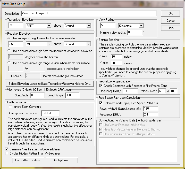
The View Shed Setup dialog provides options that allow the user to precisely setup the view shed analysis that they wish to perform.
The Description provides the user with a place to enter a name to identify this view shed analysis. This name will be displayed in the Overlay Control Center and will also be the name of the transmitter point created by the analysis for display on the map.
The Transmitter Elevation section allows the user to specify the height of the transmitter that the view shed analysis will be simulating.
The Receiver Elevation section allows the user to specify the minimum height above the ground or sea level from which the transmitter must be visible for the point to be considered visible. Most of the time you'll want to specify an elevation above ground, but specifying an elevation above sea level can be useful for aviation purposes.
Optionally, you can also specify that the receiver elevation should be calculated based on an elevation angle relative to the horizon from the transmitter. This is useful if you have something like a radar dish that points up at some angle and you want to see where the signal can be seen.
Finally, you can also specify a transmission angle range for a beam transmitted from the transmitter. Then the view shed will depict where that beam would hit the terrain surface (or some user-specified distance above the surface).
The Select Elevation Layer(s) to Base Transmitter/Receiver Heights On button displays a dialog allowing you to select which of the loaded elevation layers you want to base ground-relative transmitter and receiver heights on. The default is to use all loaded layers, but if you have a situation where you have a ground level data set loaded and perhaps another set with heights of buildings, etc., you could use this option to cause the transmitter and receiver heights to be based on the ground elevation, whereas the actual visibility of each point will use the topmost of any loaded layer.
The View Radius section allows the user to specify how far in each direction from the transmitter to check for visibility. Typically you'd want to set this to the effective range of your transmitter. If you want to ignore areas close to the transmitter, you can also specify a minimum view radius value. Use the default of 0 to include everything from the transmitter out ot the selected view radius.
The View Angle section allows the user to limit the view shed to a particular subsection of the complete radial area. The Start Angle specifies the cartographic angle at which the radial subregion begins. This angle is a cartographic angle, meaning that 0 degrees is north and angles increase clockwise. The Swept Angle specifies the number of degrees clockwise to include in the view shed. For example, if the transmitter being analyzed sweeps an arc from due south to due west, a start angle of 180 with a swept angle of 90 would be used. To perform a view shed analysis over the entire area, keep the defaults of starting at 0 degrees and sweeping through 360 degrees.
The Earth Curvature section allows the user to specify whether they want to take the curvature of the earth into account while performing the view shed analysis. In addition, when earth curvature is being used, they can specify an atmospheric correction value to be used. The atmospheric correction value is useful when determining the view shed for transmitting waves whose path is affected by the atmosphere. For example, when modeling microwave transmissions a value of 1.333 is typically used to emulate how microwaves are refracted by the atmosphere.
The Sample Spacing section allows the user to specify the spacing of elevation samples when calculating the view shed. The sample spacing controls the interval at which elevation samples are examined to determine visibility. Smaller values result in more accurate, but more slowly generated, view sheds.
The Fresnel Zone Specification section allows you to have the view shed analysis also check that a certain portion (the Percent Clear value) of the first Fresnel zone for a transmission of a particular frequency is clear. The typical standard is that good visibility requires that at least 60% (the default) of the first Fresnel zone for the specified frequency be clear of obstructions. If you specify a maximum Fresnel zone percentage clear other than 100%, only those locations where the minimum percentage of the 1st Fresnel zone that is clear is between your specified percentages will be marked as visible.
The Free Space Path Loss Calculation section allows you to display the power at any given location taking free space path loss into account. You can specify the total power from the rest of the link budget (i.e. transmission power plus antenna gain minus any other power losses excluding free space path loss) and the signal frequency. Then as you move the cursor over the view shed you can see the remaining power at the location. In addition the view shed will get more transparent as thed signal power becomes less.
The Obstructions from Vector Data section allows the user to specify whether or not loaded vector data with elevation values should be considered when performing the view shed analysis. This allows the user to use things like buildings, fence lines, towers, etc. to block portions of the view, creating a more realistic view shed. If the user elects to use vector data, they can also specify whether the elevation values stored with vector features are relative to the ground or relative to mean sea level. Typically heights for vector features are specified relative to the ground. If any area features are included and their heights are relative to the ground, the obstruction heights within those areas will be increased by the specified amount, but any receiver heights will still be based on the terrain. This makes things like wooded areas very easy to model. The Obstruction Area Features Always Hidden option allows you to specify that any locations within an obstruction area will be marked as hidden, rather than only those that actually would be hidden.
If checked, the Display Hidden Rather than Visible Areas option causes the generated view shed to cover those areas that would NOT be visible, rather than those that would be visible from the transmitter location.
If checked, the Generate Area Features in Covered Areas option specifies that view shed coverage area (polygon) featuers should be generated for those areas that are visible. These generated area features then behave just like any other vector feature and can be exported to vector formats, like Shapefiles, for use in other software.
Pressing the Select Transmitter Location... button displays a dialog that allows the user to adjust the exact transmitter coordinates from the coordinates where they clicked.
Pressing the Select Display Color... button displays a dialog that allows the user to select the color in which to display the visible areas on the map.
After setting up the view shed calculation in the dialog and pressing the OK button, the view shed analysis will be performed and when complete, the results will be displayed on the main map display as a new overlay. All visible areas within the specified radius will be displayed using the selected color. The overlay will default to being 50% translucent, allowing you to see areas underneath the view shed. You can modify the translucency of the overlay in the Overlay Control Center.
In addition, a small radio tower point will be created at the selected transmitter location. When selected using the pick tool, this point displays information about the view shed analysis as shown below.
If you would like to modify the settings used to calculate the view shed and recalculate it using currently loaded data, you can right click on the View Shed layer in the Overlay Control Center and select the option to modify the view shed.
The Image Swipe command selects the image swipe tool. This tool allows you to select a raster/image layer to swipe away by holding down the left mouse button and dragging in some direction. This allows you to easily compare overlapping layers in an interactive manner.
You will be prompted to select the raster/image layer to swipe away when activating the tool. Once active, you can change the swipe layer by right-clicking and choosing the appropriate option. To swipe, just hold down the left mouse button and drag in the desired swipe direction. When you release the mouse the swipe is reset and the entire image is displayed again.
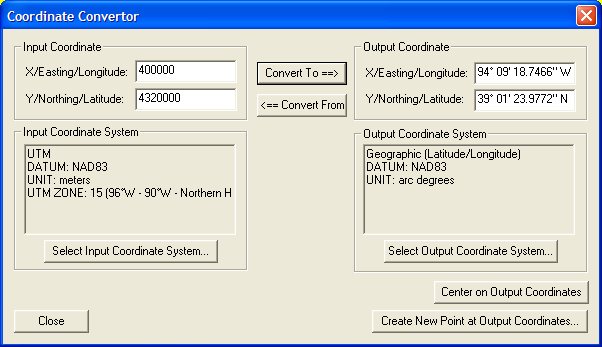
Coordinate Convertor CommandSelecting the Coordinate Convertor... menu item displays the Coordinate Convertor dialog (picture below). This dialog allows you to easily convert a coordinate in one projection/datum/unit system to another. When a conversion is made the results are automatically copied to the clipboard for easy pasting in another location using Ctrl+V. There are also buttons to allow you to easily recenter the map on the coordinates or to create a new point feature at the coordinates.

Selecting the Control Center... menu item or toolbar button displays the Overlay Control Center dialog. This dialog is the central control center for obtaining information and setting options for all loaded overlays. See the Overlay Control Center section for complete details.
Configure Command
Selecting the Configure... menu item or toolbar button displays the Configuration dialog. This dialog provides for general setup of Global Mapper display options. See the Configuration section for complete details.
Map Layout CommandSelecting the Map Layout... menu item or toolbar button displays the Map Layout dialog (pictured below). This dialog provides for setup of the map display, including specifying the placement and display of the distance scale bar, elevation legend, margins, map legend and north arrow. There are also options to save and map layout to a file and restore it later. In addition, the current map layout will be saved to any workspace files.
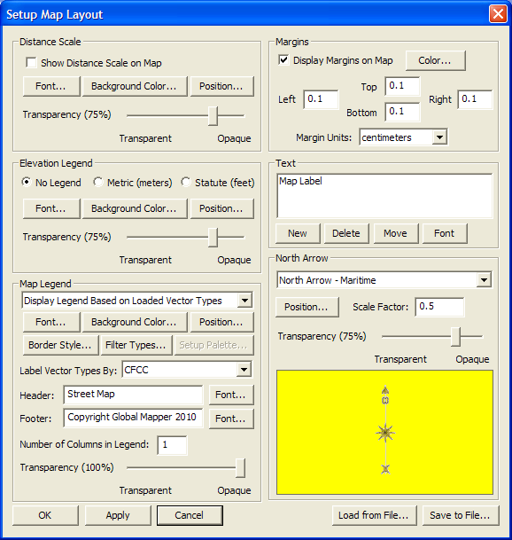
The Map Legend section allows you to setup the display of a map legend on the display. You can setup your map legend to use one of the following types: